Finite Temperature String¶

Introduction¶

Along with Nudged Elastic Band and Swarm of Trajectories, Finite Temperature String Method (FTS) is a chain-of-states method. As in other chain-of-states methods, multiple copies of a system are simulated, with each copy (“image”) corresponding to a different state of the system along some proposed transition pathway. In FTS, each image is associated with a node along a smooth curve through in collective variable space, representing a transition pathway.

The goal of FTS is to evolve the path of this smooth curve or “string” until it approximates a transition pathway by finding the principal curve, which by definition intersects each of the perpendicular hyperplanes that it passes through at the expected value of each hyperplane. As such, a principal curve is often referred to as being its own expectation. Rather than sampling along each hyperplane belonging to each node along the string, we use the Voronoi approximation introduced by Vanden-Eijnden and Venturoli in 2009 [24]. We associate each node along the string with a corresponding Voronoi cell, consisting of the region in state space where any point is closer to its origin node than any other node along the string. Each image is free to explore within the bounds of its associated Voronoi cell. To evolve the string toward its own expectation, the string is evolved toward the running averages in CV space for each image along the string.

The evolution of the string can be broken down into the following steps:

Evolve the individual images with some dynamics scheme, using the location of the initial image as a starting point. Only keep the new update at each time step if it falls within the Voronoi cell of its associated image; if the updated position leaves the Voronoi cell, the system is returned back to the state at the previous timestep.
Keep track of a running average of locations visited in CV space for each image.
Update each node on the string toward the running average while keeping the path smooth; specific equations can be found in [24].
Enforce parametrization (e.g. interpolate a smooth curve through the new node locations, and redistribute the nodes to new locations along the smooth curve such that there is equal arc length between any two adjacent nodes).
After images have been moved, their respective Voronoi cells have also changed. Check that each image still falls within the new Voronoi cell of its associated image. If the image is no longer in the correct Voronoi cell, the system must be returned to the Voronoi cell.
Return to step 1 and repeat until convergence (i.e. until change in the string falls below some tolerance criteria or stop iterating after a certain number of string method iterations)

Options & Parameters¶

The following parameters need to be set under "method" in the JSON input file:

"type" : "String"
"flavor" : "FTS"

The following options are available as FTS inputs:

centers (required): Array containing this image’s coordinates in CV space.
ksprings (required): Array of spring constants corresponding to each CV. Used to ensure that each simulation remains within its own respective Voronoi cell.
block_iterations (required): Number of integration steps to perform before updating the string. (Default: 2000)
time_step (required): Parameter used for updating the string. (\(\Delta\tau\) in [24]). (Default: 0.1)
kappa (required): Parameter used for smoothing the string. (\(\kappa\) in [24]). (Default: 0.1)
frequency (required): Frequency to perform integration; should almost always be set to 1.
max_iterations (required): Maximum number of string method iterations to perform.
tolerance (required): Array of tolerance values corresponding to each CV. Simulation will stop after tolerance criteria has been met for all CVs.
iteration: Value of initial string method iterator. (Default: 0)

Tutorial¶

Two examples for running FTS can be found in the Examples/User/FTS directory. This tutorial will go through running FTS on a 2D single particle system, using LAMMPS as the MD engine. The necessary files are found in Examples/User/FTS/2D_Particle, which should contain the following:

in.LAMMPS_2DParticle: LAMMPS input file; sets up 1 particle on a 2D surface with two Gaussian wells of different depths (at \((-0.98, -0.98)\) and \((0.98, 0.98)\)) and one Gaussian barrier at the origin.
Template_Input.json: Template JSON input containing information for one image on the string. We are looking at two CVs: x and y coordinates. We will use Input_Generator.py to use this template to create a JSON input file containing information for all string images.
Input_Generator.py: Python script for creating FTS JSON input file.

After compiling SSAGES with LAMMPS, we will use Input_Generator.py to create a JSON input file for FTS. Run this script

python Input_Generator.py

to create a file called FTS.json. A string with 16 images is initalized on the 2D surface, evenly spaced on a straight line from \((-0.98, -0.68)\) to \((0.98, 1.28)\). If you take a look at FTS.json, you will see that the location of each image along the string has been appended to the "centers" field. These center locations are listed from one end of the string to the other; the first center listed corresponds to one end of the string, and the final center listed corresponds to the opposite end of the string.

Once FTS.json has been generated, we can run the example with the following command:

mpiexec -np 16 ./ssages FTS.json

As SSAGES runs, a series of output files are generated:

log.lammps: Output from LAMMPS.
node-00xx.log: FTS output for each of the 16 nodes on the string. The first column contains the image number (0-15). The second column contains the iteration number. The remaining columns list the location of the image and the instantaneous value for each of the CVs. For this example we have two CVs (x coordinate and y coordinate), so the remaining columns are (from left to right): x coordinate of the string node, instantaneous x coordinate of the particle, y coordinate of the string node, instantaneous y coordinate of the particle.

To visualize the string, we can plot the appropriate values from the last line of each node-00xx.log file. For example, one can quickly plot the final string using gnuplot with the command

plot "< tail -n 1 node*" u 3:5

The following image shows the initial string in blue, compared with the final string plotted in green:

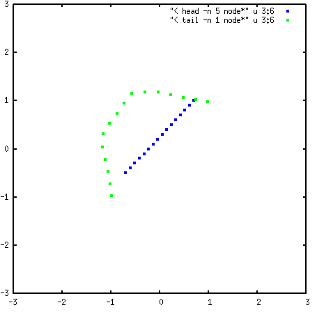
The two ends of the string have moved to the two energy minima (at \((-0.98, -0.98)\) and \((0.98, 0.98)\)), and the center of the string has curved away from the energy barrier at the origin.

Developers¶

Ashley Guo
Benjamin Sikora
Yamil J. Colón